

📈 #82 Accelerating optimization solvers with AI: the power of warmstarted linear programs
The advantage of using Graph Neural Networks in Linear Programming problems


Back in April, I received an email suggesting some exciting topics for Feasible.
The timing was perfect: I had already planned to explore similar themes, and soon afterward, someone on LinkedIn reached out asking about related content.
This sparked my interest in diving deeper into how Deep Learning integrates with Operations Research, particularly focusing on the use of Graph Neural Networks (GNNs) for optimization problems.
Today, I'm thrilled to share exactly that; and even better, it's in collaboration with a special guest: Basulaiman, Kamal.
I initially met Kamal thanks to that first email, and after a lively video call, his enthusiasm and expertise convinced me that we needed to join forces. Kamal is an independent AI consultant who expertly blends AI and optimization techniques to create intelligent, practical decision-making systems.
With experience delivering impactful solutions to companies such as Unilever, Tenaska, and Oracle, Kamal specializes in transforming cutting-edge research into tools that deliver tangible business value.
Today, he’ll share his insights into a powerful example of this approach.
I’ll leave you with him. ✨

Few real-world systems push linear programs harder than a modern electricity market: thousands of variables, strict timing, and life-or-death reliability constraints.
The stakes make it a perfect sandbox to test faster LP techniques.
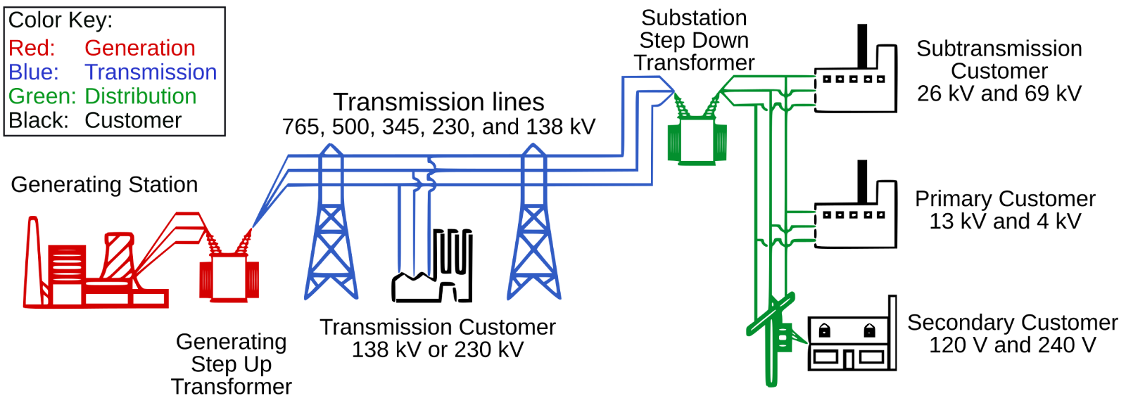
⚡️ Understanding the power grid
Before diving into the technical details, let’s first set the stage by looking at the fundamental structure of the electric power system.
The power grid can be broadly understood as having three major components: generation, transmission, and distribution.
Generation: large‐scale power plants (coal, gas, nuclear, hydro, wind, solar) produce electricity.
Transmission: a high-voltage network carries that power across regions.
Distribution: local lines and substations step voltage down and deliver electricity to homes and businesses.
To make all this possible, transformers sit at the interface between each layer. At the generation end, a generating step-up transformer boosts the voltage to very high levels for long-distance travel with minimal losses. Then, at the edge of the grid, substation step-down transformers reduce the voltage levels so that power can be safely routed through local distribution feeders and delivered to end customers.
Imagine you’re a dispatcher at the Midcontinent Independent System Operator (MISO), tasked with the challenge of keeping the lights on for millions of homes and businesses across 15 U.S. states and Manitoba, Canada. It is a high-stake balancing act as electricity can’t be economically stored at scale, so it must be generated exactly when needed, or it’s wasted.
This constant balancing act involves solving incredibly complex optimization problems. Here’s how MISO do it:
Planning Ahead:
Each morning, MISO simultaneously decides which generators to turn on for each hour of the next day and enforces a day-ahead DC Optimal Power Flow to confirm no transmission limits are violated. This is done by solving a mixed integer linear program (MILP) called Security-Constrained Unit Commitment (SCUC) problem. To ensure the system remains secure against N–1 contingencies throughout the upcoming day, the Forward Reliability Assessment and Commitment (FRAC) problem is solved. FRAC’s MILP is very similar to SCUC but with a shorter horizon and incorporates newly available weather, outage, and forecast information.Intra-Day Adjustments:
Every 15 minutes, MISO solves another MILP called Look-Ahead Commitment (LAC) problem to capture short-term ramps, fast-start resources, and intra-hour variability. LAC refines commitment and dispatch decisions made by FRAC and SCUC, ensuring that sufficient flexibility is online to meet both forecasted net load and potential contingencies. The outputs of LAC feed directly into the subsequent 5-minute Security-Constrained Economic Dispatch (SCED).
Real-Time Balancing:
Finally, every 5 minutes, MISO collects actual demand and resource data and solves its real-time Security-Constrained Economic Dispatch (SCED) problem. This Linear Program (LP) calculates exactly how much power each active plant should produce to meet demand right now, while obeying constraints like transmission line limits and safety rules. It’s a high-speed puzzle where supply must equal demand—or risk blackouts.
🌱 The renewable energy challenge: less predictable supply and demand
With solar panels and wind turbines now powering the grid, uncertainty has exploded as they depend on weather. A cloud passing over a solar farm or a sudden gust of wind can disrupt supply. On the flip side, demand used to follow predictable patterns in the past (e.g., peaks at breakfast and dinner).
But today, rooftop solar panels flood the grid with power on sunny days, and drain it when clouds roll in. Electric vehicles (EVs) charging overnight can suddenly spike demand. These fluctuations make the grid far more volatile and introduce serious operational risks if supply and demand fall out of balance:
Generator damage: large frequency deviations can overstress turbines and rotors, leading to equipment wear or catastrophic failure.
Automatic load shedding: if frequency falls too low, protective relays will shed load to protect the system, resulting in involuntary blackouts for customers.
Cascading outages: a sudden loss of one element (e.g., a line or generator) can overload others, triggering a chain reaction of failures and widespread outages.
Overheating and equipment damage: overloaded transmission lines or transformers can overheat, or flash over, causing fires or permanent equipment damage.
To guard against these risks, MISO runs thousands of “what-if” simulations each day. What many don’t realize is the sheer computational intensity of these operations.
Planning each scenario—defined by possible combinations of weather, equipment outages, and load patterns—requires solving 288 LPs per day: one for each five minutes. By aggregating results across all scenarios, MISO constructs empirical distributions of supply and demand outcomes and quantifies the probability of each risk. This statistical risk assessment ensures that the system can be pre-secured and properly resourced.
This computational burden has been a persistent bottleneck in optimization algorithms. But what if we could give these LP solvers a head start?
That's the premise behind recent innovations combining traditional mathematical optimization with Artificial Intelligence.
In this post, we'll explore a research on using neural networks to "warmstart" LP solvers, potentially transforming how we tackle complex optimization problems.
📏 The challenge of Linear Programming
Before diving into the solution details, let's understand the challenge at hand.
Linear programming involves finding the optimal value of a linear objective function subject to a set of linear constraints. One of the most common methods for solving LP problems is interior point methods (IPMs). This method cuts through the interior of the feasible region, following a central path toward the optimal solution.
While theoretically efficient, they produce dense solutions, which aren’t ideal for MIP solvers that need sparse solutions. Modern solvers often combine IPMs with simplex, using IPM solutions to warmstart simplex.

✨ The AI advantage
The practical performance of optimization algorithms depends heavily on where they start.
A good starting point can dramatically reduce computation time. Instead of relying on rule-based heuristics, AI learns patterns from historical data to predict near-optimal initial solutions.
Our initial thought was to use a "vanilla" feedforward neural network (FNN). We tried vectorizing the parameters of the LP (coefficients, constraints) and feeding them into the FNN, hoping it would spit out a good initial solution.
And... It sucked!
The predicted solutions were often infeasible, or even if feasible, they were far from optimal. The bigger problem? An FNN trained on an LP with n variables and m constraints couldn't be used for a problem with even one more variable or one less constraint. Talk about a waste of time and energy!
This led us down a different path, searching for a single neural network model that could handle varying input sizes and produce corresponding output sizes.
That's where Graph Neural Networks (GNNs) entered the picture.
GNNs are designed to process graph-structured data as inputs and predict the label of its nodes or edges. The "AHA!" moment came with the realization that an LP could be naturally encoded as a bipartite graph.
🕸️ Technical breakdown: Graph Neural Networks (GNNs) as LP whisperers
1. Encoding LPs as bipartite graphs
LPs consist of variables, constraints, and coefficients - which don't naturally fit into standard neural network architectures.
The solution? Represent each LP as a bipartite graph where variables form one set of nodes, constraints form another set of nodes, and coefficients in the constraint matrix become weighted edges connecting variables to constraints.

2. Message passing: learning LP dynamics
GNNs iteratively update node embeddings by aggregating information from neighbors. For example:
A constraint node asks variable nodes: “How much do you influence my equation?”
A variable node responds: “Based on my coefficients, here’s my best guess.”
After several iterations, the GNN predicts values of the primal and dual variables that are close to optimal.
The beauty of this approach is that it captures the complex relationships and structures within LP problems that determine which starting points will lead to faster solutions. Through repeated training on diverse problem instances, the neural network essentially "learns" the patterns that make some starting points better than others.
For more details on how GNN works, check this video:
One particularly interesting aspect is how the GNN model handles problems of different sizes. By using graph neural networks, which operate on the relational structure rather than fixed-dimensional inputs, their approach can generalize across problems of varying scales.
Though this generalization has limits!
✅ Practical results: performance gains in real-world problems
The true test of any optimization innovation is its performance on realistic problem instances.
This approach is evaluated on several LP instances of real-world problems, including economic dispatch, market clearing, load matching, relaxed travelling salesman problem (TSP), relaxed set covering, and relaxed unit commitment.
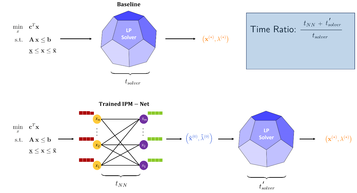
The results demonstrate that this learning-to-warmstart approach consistently yields solutions with an optimality gap below 7% and constraint violations under 0.3%. These results translate into an average of 8% reduction in runtime compared to state-of-the-art commercial solvers like Gurobi.
What's particularly significant is that these improvements come essentially "for free" after the initial training investment.
Once trained, the GNN model makes its predictions in milliseconds, adding negligible overhead to the solution process.
🔬 Limitations and opportunities
No approach is without limitations, so here is a highlight of the main challenges that remain to be addressed:
Infeasibility issues: the learning-to-warmstart approach sometimes predicts infeasible initial solutions (up to 10.5% of cases), which are discarded by the solver. Exploring feasibility restoration techniques could help mitigate the infeasibility issues by projecting the predicted initial solutions back to the feasible region. Check this paper for an example of how feasibility restoration is implemented to warmstart the Simplex algorithm.
Limited generalization: models trained on one type of problem (e.g., TSP) didn't transfer well to different problem types (e.g., Set Covering), suggesting that problem-specific training is still necessary.
Limited scaling to larger instances: model performance declined when evaluated on instances larger than those used for training. The larger the test instance relative to those seen during training, the more noticeable the performance degradation.
🧭 Business implications for adopting this approach
The practical implications of this approach unlock significant cost savings and competitive advantages. Consider the following potential implications.
By reducing solver runtime, organizations can significantly reduce solver license costs while maintaining problem-solving capacity.
Faster computations enable real-time decision-making, allowing businesses to adapt instantly to market shifts (e.g., supply chain disruptions, demand spikes, or price volatility), avoiding costly delays and capitalizing on fleeting opportunities.
This agility enhances brand reputation as a leader in innovation and reliability, attracting clients and partners seeking cutting-edge efficiency.
Combined, these efficiencies translate to increased market share, as competitors lag in speed and adaptability, while cost savings from licenses and operational gains fuel reinvestment in innovation.
In fast-moving industries like energy trading, speed isn’t just efficiency, it is a catalyst for sustained growth and competitive dominance.
🏁 Conclusions
The marriage of Machine Learning and Mathematical Optimization represents one of the most exciting frontiers in computational problem-solving.
By teaching neural networks to understand the structure of optimization problems, researchers are creating systems that combine the mathematical rigor of traditional algorithms with the pattern recognition abilities of AI.
What is particularly exciting is how this approach challenges the traditional dichotomy between exact and approximate methods. Instead of choosing between slow-but-optimal solvers and fast-but-imprecise heuristics, Machine Learning bridges the gap, accelerating exact methods to get great speed-ups.
Top commercial solver providers must adopt learning-to-warmstart techniques within their MIP engine to retain their market dominance. Open-source and lower-cost alternatives are already leveraging AI to close the performance gap with premium solvers. For instance, NVIDIA is on its mission to deliver cuOpt, a GPU-Accelerated and AI-guided optimization engine to solve large-scale problems.
If established players fail to innovate, they risk being displaced by agile competitors offering comparable speed and accuracy at a fraction of the cost. For commercial solvers, embedding AI-driven warmstarting isn’t just an upgrade, it is a survival strategy in an era where efficiency and adaptability are crucial.
As real-world systems keep getting more complicated, the need for faster ways to solve large optimization problems grows quickly.
Whether it is untangling messy supply chains, balancing power grids spread across regions, or deciding where to send medical supplies when hospitals are overwhelmed, being able to find the best solutions fast isn’t just helpful, it is becoming essential.
Let’s keep optimizing,
Kamal.
🗞️ Other related posts people like


 | A guest post by
|
Good Luck!
Great article, best wishes Kamal